Autodiff for Multilevel Optimization

In this paper, we focus in particular on gradient-based multilevel optimization, rather than zeroth-order methods like Bayesian optimization, in order to efficiently scale to high-dimensional problems. Essentially, gradient-based multilevel optimization calculates gradients of the cost function \(\mathcal{C}_k(\theta_k, \mathcal{U}_k, \mathcal{L}_k)\) with respect to the corresponding parameter \(\theta_k\), with which gradient descent is performed to solve for optimal parameters \(\theta_k^*\) for every problem \(P_k\). Since optimal parameters from lower level problems (i.e. \(\theta_l^*\in\mathcal{L}_k\)) can be functions of \(\theta_k$\), \(\frac{d\mathcal{C}_k}{d\theta_k}\) can be expanded using the chain rule as follows:

\[\begin{flalign} &&\frac{d\mathcal{C}_k}{d\theta_k} = \textcolor{brown}{\underbrace{\frac{\partial\mathcal{C}_k}{\partial\theta_k}}_\text{direct gradient}} + \sum_{\theta_l^*\in\mathcal{L}_k}\textcolor{blue}{\underbrace{\frac{d\theta_l^*}{d\theta_k}}_\text{best-response Jacobian}} \times\textcolor{brown}{\underbrace{\frac{\partial\mathcal{C}_k}{\partial\theta_l^*}}_\text{direct gradient}}&&\text{(1)} \end{flalign}\]

While calculating direct gradients is straightforward with existing automatic differentiation frameworks such as PyTorch, a major difficulty in gradient-based MLO lies in best-response Jacobian (i.e. \(\frac{d\theta_l^*}{d\theta_k}\)), which will be discussed in depth in the following subsections. Once gradient calculation is enabled, gradient-based optimization is executed from lower-level problems to upper-level problems in a topologically reverse order, reflecting the underlying hierarchy.

Dataflow Graph for Multilevel Optimization

One may observe that the best-response Jacobian term in Equation (1) is expressed with a total derivative instead of a partial derivative. This is because \(\theta_k\) can affect \(\theta_l^*\) not only through a direct interaction, but also through multiple indirect interactions via other lower-level optimal parameters. For example, consider the four-problem MLO program illustrated in Figure 1. Here, the parameter of Problem 4 (\(\theta_{p_4}\)) affects the optimal parameter of Problem 3 (\(\theta_{p_3}^*\)) in two different ways: (1) \(\theta_{p_4} \rightarrow \theta_{p_3}^*\) and (2) \(\theta_{p_4} \rightarrow \theta_{p_1}^* \rightarrow \theta_{p_3}^*\). In general, we can expand the best-response Jacobian \(\frac{d\theta_l^*}{d\theta_k}\) in Equation (1) by applying the chain rule for all paths from \(\theta_k\) to \(\theta_l^*\) as:

\[\begin{flalign} &&\frac{d\mathcal{C}_k}{d\theta_k} = \frac{\partial\mathcal{C}_k}{\partial\theta_k} + \sum_{\theta_l^*\in\mathcal{L}_k}\sum_{q\in\mathcal{Q}_{k,l}}\Bigg(\textcolor{red}{\underbrace{\frac{\partial\theta_{q(1)}^*}{\partial\theta_k}}_\text{upper-to-lower}}\times \Bigg(\prod_{i=1}^{\text{len}(q)-1}\textcolor{green}{\underbrace{\frac{\partial\theta_{q(i+1)}^*}{\partial\theta_{q(i)}^*}}_\text{lower-to-upper}}\Bigg)\times\frac{\partial\mathcal{C}_k}{\partial\theta_l^*}\Bigg)&&\text{(2)} \end{flalign}\]

where \(\mathcal{Q}_{k, l}\) is a set of paths from \(\theta_k\) to \(\theta_l^*\), and \(q(i)\) refers to the index of the \(i\)-th problem in the path \(q\) with the last point being \(\theta_l^*\). Replacing a total derivative term in Equation (1) with a product of partial derivative terms using the chain rule allows us to ignore indirect interactions between problems, and only deal with direct interactions.

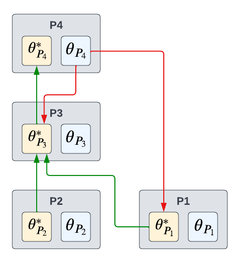
Figure 1. A dataflow graph example of multilevel optimization

To formalize the path finding problem, we develop a novel dataflow graph for MLO. Unlike traditional dataflow graphs with no predefined hierarchy among nodes, a dataflow graph for multilevel optimization has two different types of directed edges: lower-to-upper and upper-to-lower. Each of these directed edges is respectively depicted with \(\textcolor{green}{\text{green}}\) and \(\textcolor{red}{\text{red}}\) arrows in Figure 1. Essentially, a lower-to-upper edge represents the directed dependency between two optimal parameters (i.e. \(\theta_i^* \rightarrow \theta_j^*$ with $i<j\)), while an upper-to-lower edge represents the directed dependency between nonoptimal and optimal parameters (i.e. \(\theta_i \rightarrow \theta_j^*\) with \(i>j\)). Since we need to find paths from the nonoptimal parameter \(\theta_k\) to the optimal parameter \(\theta_l^*\), the first directed edge must be an upper-to-lower edge \(\textcolor{red}{\text{(red)}}\), which connects \(\theta_k\) to some lower-level optimal parameter. Once it reaches the optimal parameter, it can only move through optimal parameters via lower-to-upper edges \(\textcolor{mygreen}{\text{(green)}}\) in the dataflow graph. Therefore, every valid path from \(\theta_k\) to \(\theta_l^*\) will start with an upper-to-lower edge, and then reach the destination only via lower-to-upper edges. The best-response Jacobian term for each edge in the dataflow graph is also marked with the corresponding color in Equation (2). We implement the above path finding mechanism with a modified depth-first search algorithm in Betty.

Gradient Calculation with Best-Response Jacobian

Automatic differentiation for MLO can be realized by calculating Equation (2) for each problem \(P_k\) (\(k=1,\cdots,n\)). However, a naive calculation of Equation (2) could be computationally onerous as it involves multiple matrix multiplications with best-response Jacobians, of which the computational complexity is \(\mathcal{O}(n^3)\). To alleviate this issue, we observe that the rightmost term in Equation (2) is a vector, which allows us to reduce the computational complexity of Equation (2) to \(\mathcal{O}(n^2)\) by iteratively performing matrix-vector multiplication from right to left (or, equivalently, reverse-traversing a path \(q\) in the dataflow graph). As such, matrix-vector multiplication between the best-response Jacobian and a vector serves as a base operation of efficient automatic differentiation for MLO. Mathematically, this problem can be simply written as follows:

\[\begin{split}\begin{flalign} &&\text{Calculate}\,:\quad&\frac{\partial w^*(\lambda)}{\partial \lambda}\times v &&\quad\quad\quad\text{(3)}\\ &&\text{Given}\,:\quad&w^*(\lambda) = \underset{w}{\mathrm{argmin}}\;\mathcal{C}(w, \lambda) &&\quad\quad\quad\text{(4)} \end{flalign}\end{split}\]

Two major challenges in the above problems are: (1) approximating the solution of the optimization problem (i.e. \(w^*(\lambda)\)), and (2) differentiating through the (approximated) solution.

In practice, an approximation of \(w^*(\lambda)\) is typically achieved by unrolling a small number of gradient steps, which can significantly reduce the computational cost. While we could potentially obtain a better approximation of \(w^*(\lambda)\) by running gradient steps until convergence, this procedure alone can take a few days (or even weeks) when the underlying optimization problem is large-scale (e.g. ImageNet or BERT).

Once \(w^*(\lambda)\) is approximated, matrix-vector multiplication between the best-response Jacobian \(\frac{dw^*(\lambda)}{d\lambda}\) and a vector \(v\) is popularly obtained by either iterative differentiation (ITD) or approximate implicit differentiation (AID). This problem has been extensively studied in bilevel optimization literature [Grazzi et al., Franceschi et al., Liu et al., Lorraine et al., Maclaurin et al.], and we direct interested readers to the original papers,

Here, we provide several insights about each algorithm here. Roughly speaking, ITD differentiates through the optimization path of Equation (4), whereas AID only depends on the (approximated) solution \(w^*(\lambda)\). Due to this difference, AID is oftentimes considered to be more memory efficient than ITD. The same observation has also been made based on a theoretical analysis in Ji et al.. Moreover, a dependency to the optimization path requires ITD to track the intermediate states of the parameter during optimization, but existing frameworks like PyTorch override such intermediate states through the use of stateful modules and in-place operations in the optimizer. Hence, ITD requires patching modules and optimizers to support intermediate state tracking as well.

Overall, AID provides two important benefits compared to ITD: it can allow better memory efficiency, and use native modules/optimizers of existing frameworks. Thus, in Betty we also primarily direct our focus on AID algorithms while also providing an implementation of ITD for completeness. Currently available best-response Jacobian calculation algorithms in Betty include (1) ITD with reverse-mode automatic differentiation [Finn et al.], (2) AID with Neumann series [Lorraine et al.], (3) AID with conjugate gradient [Rajeswaran et al.], and (4) AID with finite difference [Liu et al.]. Users can choose whichever algorithm is most-appropriate for each problem in their MLO program, and the chosen algorithm is used to perform the matrix-vector multiplication with best-response Jacobians in Equation (2) for the corresponding problem based on the dataflow graph, accomplishing automatic differentiation for MLO. By default, Betty uses (4) AID with finite difference (i.e. darts), as we empirically observe that darts achieves the best memory efficiency, training wall time, and final accuracy across a wide range of tasks.

In general, the above automatic differentiation technique for multilevel optimization has a lot in common with reverse-mode automatic differentiation (i.e. backpropagation) in neural networks. In particular, both techniques achieve gradient calculation by iteratively multiplying Jacobian matrices while reverse-traversing dataflow graphs. However, the dataflow graph of MLO has two different types of edges, due to its unique constraint criteria, unlike that of neural networks with a single edge type. Furthermore, Jacobian matrices in MLO are generally approximated with ITD or AID while those in neural networks can be analytically calculated.